All the code here is derived from the legendary book ISRL 2nd edition’s chapter 8 “Decision Trees”. Its sometimes a wonder how elegant the base R language can be. The ISRL lab rarely mentions tidyverse syntax but yet manages to make the code so easy to read. The more you learn!🤓

Quick Revision

In $Bagging$ , the trees are grown independently on random samples of the observations. Consequently, the trees tend to be quite similar to each other. Thus, bagging can get caught in local optima and can fail to thoroughly explore the model space
In $Random Forest$, the trees are grown independently on random samples of the observations. However, each split on each tree is performed on random subset of predictors, thereby decorrelating the trees and leading to a better exploration relative to bagging. Both bagging & RF are ensemble methods which makes prediction from average of regression trees. Both also use bootstrap sampling.
In $Boosting$, we only use the original data and don’t draw random samples. The trees are grown successively using a “slow” learning approach; each new tree is fit to the signal that is left over from the earlier trees. Boosting is an ensemble method that uses weighted sum and doesn’t involve bootstrap sampling as the trees are fitted on a modified version of the original dataset.
In $BART$, we only use the original data and we grow the trees successively. However each tree is perturbed in order to avoid local minima. BART is related to the Boosting & RF — each tree is created in a random manner like bagging & RF and each tree tries to capture some signal not yet accounted for in the current model like Boosting. BART tries to improve the partial residual of current tree by slightly modifying the previous iteration (changing the structure by altering number of nodes)

Code

library(tree)
library(ISLR2)

In today’s lab, we will be using the Carseats dataset from the ISLR2 package.

Code

str(Carseats)

'data.frame':   400 obs. of  11 variables:
 $ Sales      : num  9.5 11.22 10.06 7.4 4.15 ...
 $ CompPrice  : num  138 111 113 117 141 124 115 136 132 132 ...
 $ Income     : num  73 48 35 100 64 113 105 81 110 113 ...
 $ Advertising: num  11 16 10 4 3 13 0 15 0 0 ...
 $ Population : num  276 260 269 466 340 501 45 425 108 131 ...
 $ Price      : num  120 83 80 97 128 72 108 120 124 124 ...
 $ ShelveLoc  : Factor w/ 3 levels "Bad","Good","Medium": 1 2 3 3 1 1 3 2 3 3 ...
 $ Age        : num  42 65 59 55 38 78 71 67 76 76 ...
 $ Education  : num  17 10 12 14 13 16 15 10 10 17 ...
 $ Urban      : Factor w/ 2 levels "No","Yes": 2 2 2 2 2 1 2 2 1 1 ...
 $ US         : Factor w/ 2 levels "No","Yes": 2 2 2 2 1 2 1 2 1 2 ...

Creating a column called High which takes a Y/N value depending on the sales and then merge it with the Carseats df.

Code

attach(Carseats)
High <- factor(ifelse(Sales <= 8, "No", "Yes"))
Carseats <- data.frame(Carseats, High)

Fitting Classification Trees on `Carseats`

Creating a classification tree to predict High using all variables except Sales

Code

set.seed(1)
tree.carseats <- tree(High ~ .-Sales, data = Carseats)
summary(tree.carseats)


Classification tree:
tree(formula = High ~ . - Sales, data = Carseats)
Variables actually used in tree construction:
[1] "ShelveLoc"   "Price"       "Income"      "CompPrice"   "Population" 
[6] "Advertising" "Age"         "US"         
Number of terminal nodes:  27 
Residual mean deviance:  0.4575 = 170.7 / 373 
Misclassification error rate: 0.09 = 36 / 400

Misclassification error of 9% is a good fit. Let’s try plotting it

Code

plot(tree.carseats)
text(tree.carseats, pretty  =0 )

Splitting and fitting the model

Code

set.seed(2)
train <- sample(1:nrow(Carseats), 200)
Carseats.test <- Carseats[-train,]
High.test <- High[-train]
tree.carseats <- tree(High ~ .-Sales, data = Carseats, 
                      subset = train)

checking the top few rows of predicted columns

Code

tree.predict <- predict(tree.carseats, Carseats.test, 
                        type = "class") #type is needed to declare classification model
head(tree.predict)

[1] Yes No  No  Yes No  No 
Levels: No Yes

Comparing predicted with actual values

Code

table(tree.predict, High.test)

            High.test
tree.predict  No Yes
         No  104  33
         Yes  13  50

What’s the accuracy?

Code

(104+50)/200

[1] 0.77

77% Accuracy

Pruning the tree for improved classification

To improve the accuracy, lets attempt to prune the tree. For this cv.tree() function is used to determine the optimal level of tree complexity. Here the FUN argument is taken as prune.misclass to indicate that the cross-validation and tree pruning should be guided by the classification error instead of the default deviance.

Code

set.seed(7)
cv.carseats <- cv.tree(tree.carseats, FUN = prune.misclass)
names(cv.carseats)

[1] "size"   "dev"    "k"      "method"

Note to self:

k is the regularisation parameter $\alpha$ (alpha)
size is # of terminal nodes for each tree
dev is the number of cross-validation errors

Code

cv.carseats

$size
[1] 21 19 14  9  8  5  3  2  1

$dev
[1] 75 75 75 74 82 83 83 85 82

$k
[1] -Inf  0.0  1.0  1.4  2.0  3.0  4.0  9.0 18.0

$method
[1] "misclass"

attr(,"class")
[1] "prune"         "tree.sequence"

Visualising the tree. The classification error is least (74) at size = 9

Code

par(mfrow = c(1,2))
plot(cv.carseats$size, cv.carseats$dev, type = "b")
plot(cv.carseats$k, cv.carseats$dev, type = "b")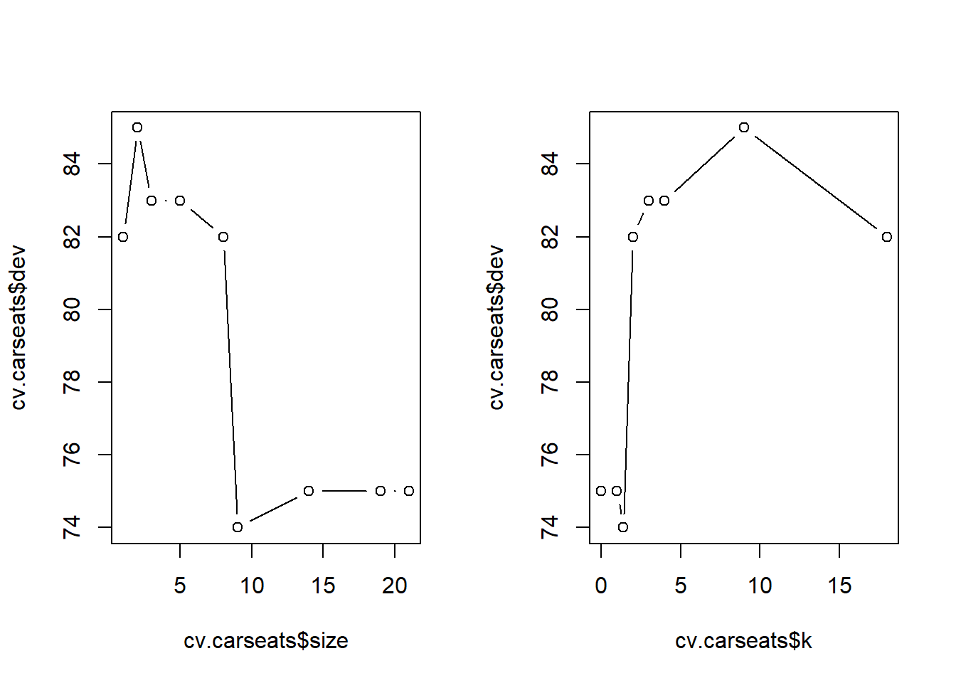

Relation between Deviance with tree size & regularisation parameter

Using the prune.misclass() function to prune the tree to the 9-node specification.

Code

prune.carseats= prune.misclass(tree.carseats, best = 9)
plot(prune.carseats)
text(prune.carseats, pretty = 0)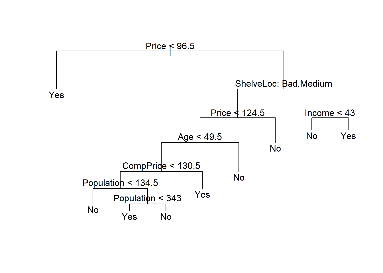

Checking the accuracy in the good-old fashioned way (its really that simple!)🤓

Code

prune.tree.pred <- predict(prune.carseats, Carseats.test, type = "class")
table(prune.tree.pred, High.test)

               High.test
prune.tree.pred No Yes
            No  97  25
            Yes 20  58

So what’s the accuracy?

Code

(97+58)/200

[1] 0.775

77.5% which is slightly better than the non-pruned tree. Not bad.

Key Takeaways

Without tuning the model, the default DT algo creates a tree with 27 nodes
deviance measured as a result of changing the number of nodes indicates the best DT of 9 nodes.
The code needed to write this is surprisingly simple. However, the tidymodels interface allows for managing the resulting output and models in a more structured way.

Fitting regression trees on `Boston` dataset

Boston dataset contains housing values of 506 suburbs of Boston. We are trying to predict the median value of the owner-occupied homes medv

Code

str(Boston)

'data.frame':   506 obs. of  13 variables:
 $ crim   : num  0.00632 0.02731 0.02729 0.03237 0.06905 ...
 $ zn     : num  18 0 0 0 0 0 12.5 12.5 12.5 12.5 ...
 $ indus  : num  2.31 7.07 7.07 2.18 2.18 2.18 7.87 7.87 7.87 7.87 ...
 $ chas   : int  0 0 0 0 0 0 0 0 0 0 ...
 $ nox    : num  0.538 0.469 0.469 0.458 0.458 0.458 0.524 0.524 0.524 0.524 ...
 $ rm     : num  6.58 6.42 7.18 7 7.15 ...
 $ age    : num  65.2 78.9 61.1 45.8 54.2 58.7 66.6 96.1 100 85.9 ...
 $ dis    : num  4.09 4.97 4.97 6.06 6.06 ...
 $ rad    : int  1 2 2 3 3 3 5 5 5 5 ...
 $ tax    : num  296 242 242 222 222 222 311 311 311 311 ...
 $ ptratio: num  15.3 17.8 17.8 18.7 18.7 18.7 15.2 15.2 15.2 15.2 ...
 $ lstat  : num  4.98 9.14 4.03 2.94 5.33 ...
 $ medv   : num  24 21.6 34.7 33.4 36.2 28.7 22.9 27.1 16.5 18.9 ...

Creating the training set for Boston which is half the size of the original

Code

set.seed(1)
train.boston <- sample(1:nrow(Boston), nrow(Boston)/2)

Building the tree

Code

tree.boston <- tree(medv ~ ., data = Boston, subset = train.boston)
summary(tree.boston)


Regression tree:
tree(formula = medv ~ ., data = Boston, subset = train.boston)
Variables actually used in tree construction:
[1] "rm"    "lstat" "crim"  "age"  
Number of terminal nodes:  7 
Residual mean deviance:  10.38 = 2555 / 246 
Distribution of residuals:
    Min.  1st Qu.   Median     Mean  3rd Qu.     Max. 
-10.1800  -1.7770  -0.1775   0.0000   1.9230  16.5800

only 4 predictors rm, lstat, crim, age were used. (wonder why?) Plotting the decision tree

Code

plot(tree.boston)
text(tree.boston, pretty = 0)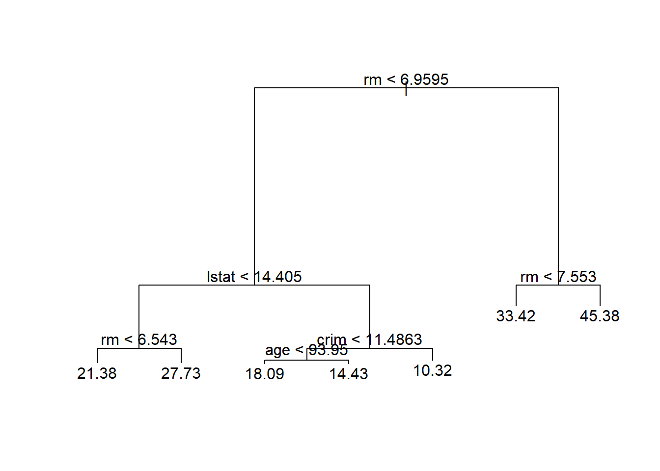

Representing the decision tree with 7 nodes

Making the predictions

Code

yhat <- predict(tree.boston, newdata = Boston[-train.boston,])
test.boston <- Boston[-train.boston,"medv"]

plot(yhat, test.boston)
abline(0,1, col = "red")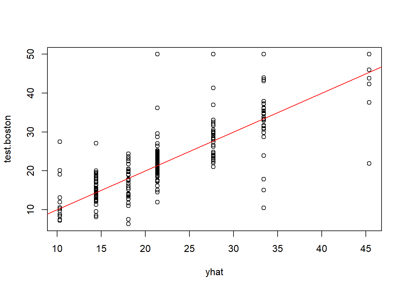

This plot visualises the Predicted v/s Actuals for Boston test data

Mean Square Error is defined as \[MSE = \frac{1}{n} \sum_{i=1}^{n}(y_i - \hat{y_i})^2\]

Code

mean((yhat - test.boston)^2)

[1] 35.28688

RMSE which uses the same units as the output variable is:

Code

(mean((yhat - test.boston)^2))^0.5

[1] 5.940276

Key Takeaways:

As the SD is the same units as the outcome variable, we can say that this model leads to predictions which on an average are within ±$5940 of the true median home value. Can we do better? Let’s keep digging

Regression using Bagging & Random Forests

Note: Bagging is a special case of Random Forest where $m = p$. The randomForest() function can be used for evaluating predictions from both bagging & RF. So first up is the Bagging process

$m$ = sample number of predictors

$p$ = total number of available predictors

Bagging

importance parameter here will compute and return the importance measures of each predictor variable. Importance measures provide a way to assess the relative importance of each predictor variable in the random forest model, based on the decrease in accuracy that occurs when that variable is excluded from the model. This increases the runtime significantly on large datasets

Code

library(randomForest)
set.seed(1)
bag.boston <- randomForest(medv ~ . , data = Boston, 
                           subset = train.boston, 
                           mtry = 12, # m = p
                           importance = T)
bag.boston


Call:
 randomForest(formula = medv ~ ., data = Boston, mtry = 12, importance = T,      subset = train.boston) 
               Type of random forest: regression
                     Number of trees: 500
No. of variables tried at each split: 12

          Mean of squared residuals: 11.40162
                    % Var explained: 85.17

Code

yhat.bag <- predict(bag.boston, newdata = Boston[-train.boston, ])
plot(yhat.bag, test.boston)
abline(0,1,col = "red")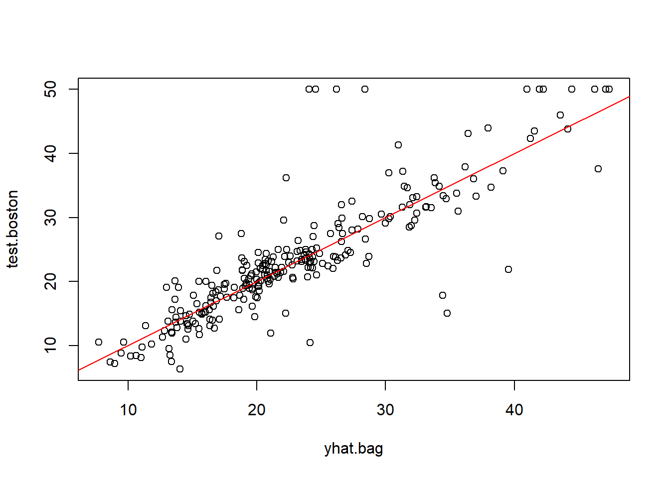

Predicted v/s Actuals for Boston test data using Bagging

What’s the accuracy here? Checking the MSE

Code

mean((yhat.bag - test.boston)^2)

[1] 23.41916

And square root of MSE or RMSE is:

Code

(mean((yhat.bag - test.boston)^2))^0.5

[1] 4.839335

That’s $4839 which is better than $ 5940 derived from the 7-node decision tree discussed in Key Takeaways. Moving to Random Forest now.

Random Forest

Its the same code, but we alter the number of predicted variables to $m= 6$ which is the mtry parameter

Default settings for randomForest()

for regression analysis, $m = p/3$

for classification analysis, $m = \sqrt p$

Code

set.seed(1)
rf.boston <- randomForest(medv ~ . , data = Boston, 
                           subset = train.boston, 
                           mtry = 6, # m = p/2
                           importance = T)
rf.boston


Call:
 randomForest(formula = medv ~ ., data = Boston, mtry = 6, importance = T,      subset = train.boston) 
               Type of random forest: regression
                     Number of trees: 500
No. of variables tried at each split: 6

          Mean of squared residuals: 10.09466
                    % Var explained: 86.87

Code

yhat.rf <- predict(rf.boston, newdata = Boston[-train.boston, ])
plot(yhat.rf, test.boston)
abline(0,1,col = "red")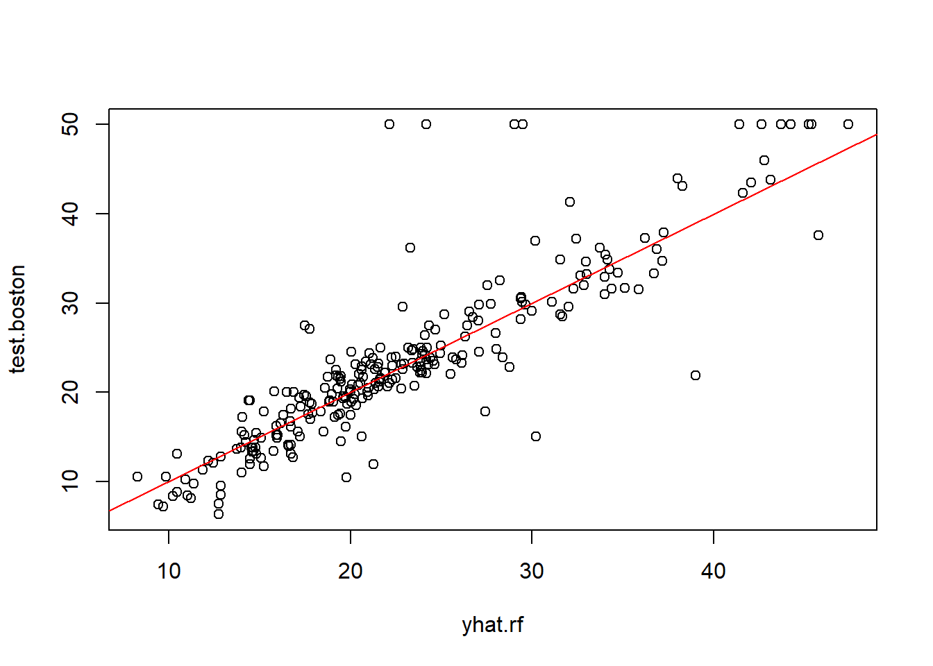

Predicted v/s Actuals for Boston test data using RandomForest

What’s the MSE here?

Code

mean((yhat.rf - test.boston)^2)

[1] 20.06644

.. and therefore RMSE is:

Code

mean((yhat.rf - test.boston)^2)^0.5

[1] 4.479558

That’s ±$4480 from the mean predicted values - which is better than $4839 by using the Bagging method.

Before moving ahead, we can also check the importance() function to determine key predictors

Code

importance(rf.boston)

          %IncMSE IncNodePurity
crim    19.435587    1070.42307
zn       3.091630      82.19257
indus    6.140529     590.09536
chas     1.370310      36.70356
nox     13.263466     859.97091
rm      35.094741    8270.33906
age     15.144821     634.31220
dis      9.163776     684.87953
rad      4.793720      83.18719
tax      4.410714     292.20949
ptratio  8.612780     902.20190
lstat   28.725343    5813.04833

What are these columns?

%IncMSE: Avg decrease in accuracy of predictions on out-of-bag samples when given variable is calculated
IncNodePurity:Total decrease in node purity that results from split on that variable averaged over all trees.
- in regression trees, the node impurity measured by the training Residual Sum of Squares(RSS)
- in classification trees, it is the deviance

Code

varImpPlot(rf.boston)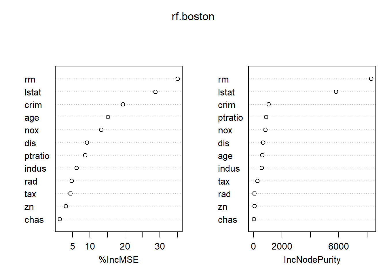

This shows that the two most important variables are rm (average number of rooms per dwelling) and lstat (lower status of the population in %)

Boosting

Using the gbm package (Gradient Boosting Model) for boosted trees. Few notes:

distribution = "gaussian" is considered for regression trees. For classification, it should be distribution = "bernoulli"
n.trees = 5000 is the number of trees we want to iterate over
interaction.depth = 4 limits the depth of each tree

Code

library(gbm) #Gradient Boosting Models
set.seed(1)
boost.boston <- gbm(medv ~ ., data = Boston[train,], 
                    distribution = "gaussian",
                    n.trees = 5000,
                    interaction.depth = 4)
summary(boost.boston)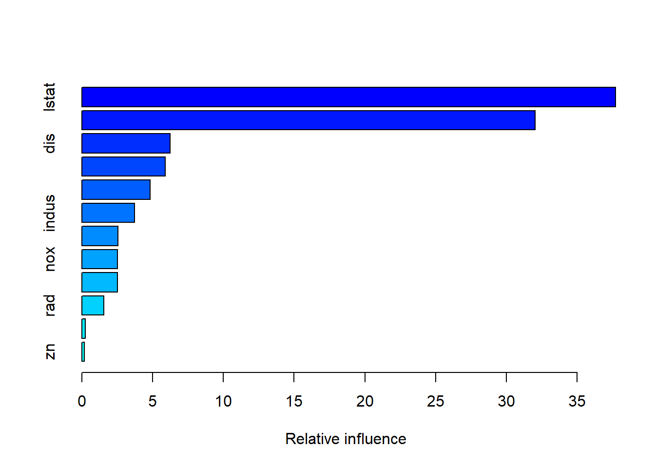

            var    rel.inf
lstat     lstat 37.7145639
rm           rm 32.0396810
dis         dis  6.2532723
crim       crim  5.9078403
age         age  4.8163355
indus     indus  3.7365846
tax         tax  2.5457121
nox         nox  2.5286998
ptratio ptratio  2.5091014
rad         rad  1.5427771
chas       chas  0.2451445
zn           zn  0.1602876

As seen earlier, lm and rstat show up as the most important variables.

partial dependence plots

By plotting the partial dependence of rm and lstat on outcome variable, we see that

rm has a direct relation viz. more the number of rooms, higher the price increases
lstat has an inverse relation viz. higher the lower stata in the neighbourhood, lower the price

Code

par(mfrow = c(1,2))
plot(boost.boston, i = "rm")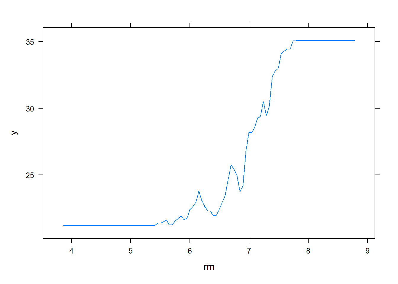

Code

plot(boost.boston, i = "lstat")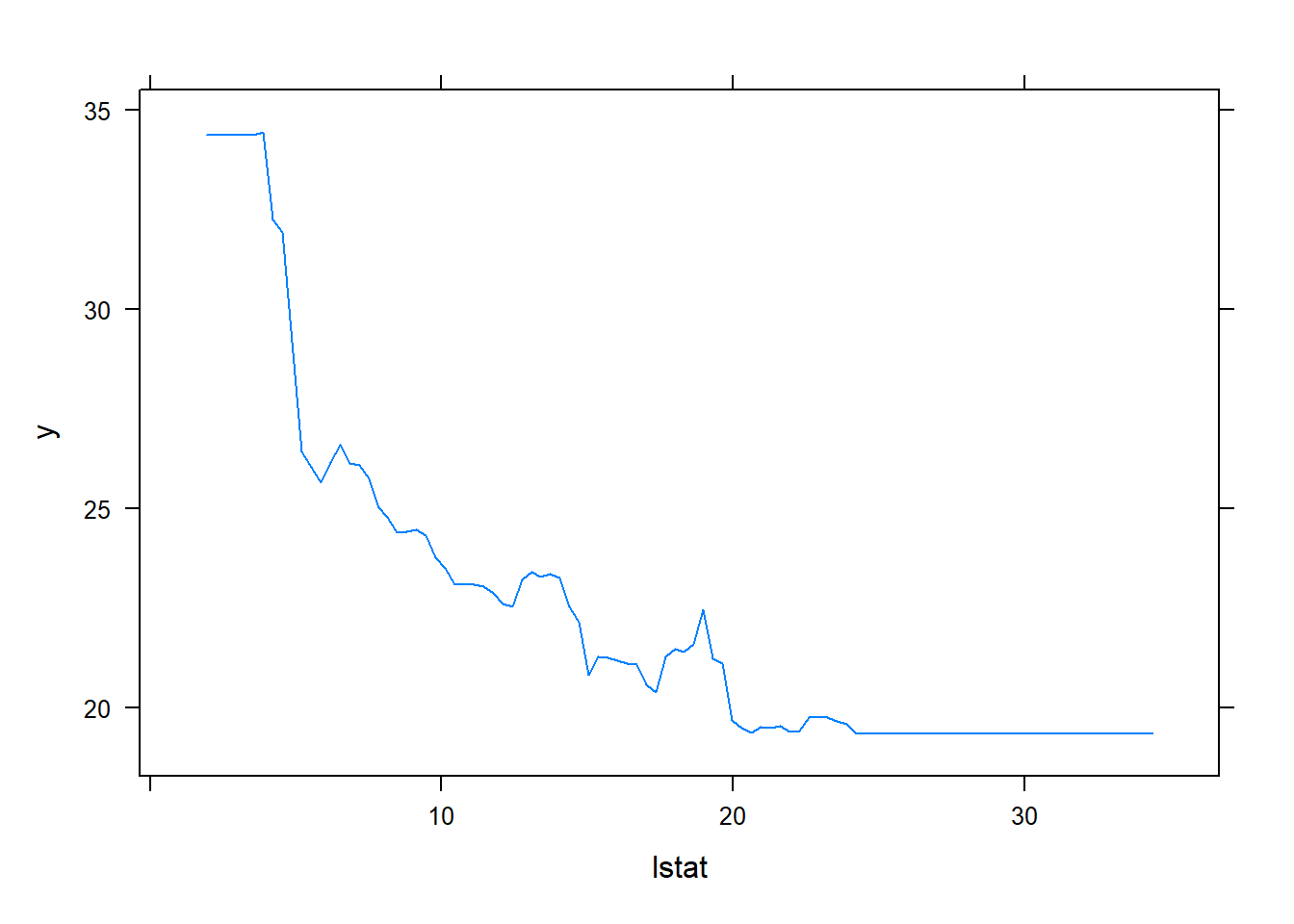

Predictions

Code

yhat.boost <- predict(boost.boston, newdata = Boston[-train.boston,], 
                      n.trees = 5000)

#| fig-cap: "Predicted v/s Actuals for Boston test data using Boosted RF"
#| fig-cap-location: top
plot(yhat.boost, test.boston)
abline(0,1,col = "red")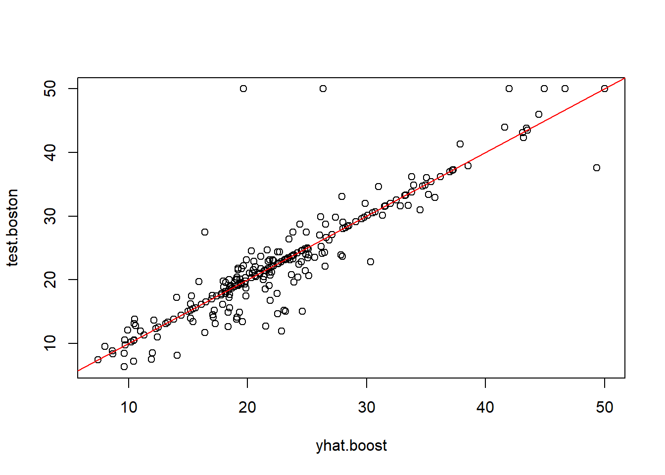

Figure looks so much better. testing the accuracy now. starting with the MSE

Code

mean((yhat.boost - test.boston)^2)

[1] 12.98195

Wow.. that’s significantly lower. How about the RMSE?

Code

mean((yhat.boost - test.boston)^2)^0.5

[1] 3.603047

Amazing. This means our predicted value on an average is ±$3603 from the actual which is a signifcant improvement from the RMSE calculated by Random Forest ±$4480

Adding regularisation parameter 𝛌

Also referred as the shrinkage parameter, the default value is 0.001 but we will change this to 0.01

Code

set.seed(1)
boost.boston2 <- gbm(medv ~ ., data = Boston[train,], 
                    distribution = "gaussian",
                    n.trees = 5000,
                    interaction.depth = 4, 
                    shrinkage = 0.01)
yhat.boost2 <- predict(boost.boston2, newdata = Boston[-train.boston,], 
                      n.trees = 5000)

The resulting MSE therefore is calculated as:

Code

mean((yhat.boost2 - test.boston)^2)^0.5

[1] 3.593472

Now we’ve got it even lower at ±$3593

Bayesian Additive Regression Trees

The function gbart() is used for regression analysis. This syntax slightly reminds me of the python syntax as we’re back to creating matrices for each test, train, x & y.

Code

library(BART)
x_BART <- Boston[,1:12]
y_BART <- Boston[,"medv"]

xtrain_BART <- x_BART[train.boston, ]
ytrain_BART <- y_BART[train.boston]

xtest_BART <-  x_BART[-train.boston, ]
ytest_BART <- y_BART[-train.boston]

Creating the model now:

Code

set.seed(1)
bart_model <- gbart(xtrain_BART, ytrain_BART, x.test = xtest_BART)

*****Calling gbart: type=1
*****Data:
data:n,p,np: 253, 12, 253
y1,yn: 0.213439, -5.486561
x1,x[n*p]: 0.109590, 20.080000
xp1,xp[np*p]: 0.027310, 7.880000
*****Number of Trees: 200
*****Number of Cut Points: 100 ... 100
*****burn,nd,thin: 100,1000,1
*****Prior:beta,alpha,tau,nu,lambda,offset: 2,0.95,0.795495,3,3.71636,21.7866
*****sigma: 4.367914
*****w (weights): 1.000000 ... 1.000000
*****Dirichlet:sparse,theta,omega,a,b,rho,augment: 0,0,1,0.5,1,12,0
*****printevery: 100

MCMC
done 0 (out of 1100)
done 100 (out of 1100)
done 200 (out of 1100)
done 300 (out of 1100)
done 400 (out of 1100)
done 500 (out of 1100)
done 600 (out of 1100)
done 700 (out of 1100)
done 800 (out of 1100)
done 900 (out of 1100)
done 1000 (out of 1100)
time: 9s
trcnt,tecnt: 1000,1000

Computing the test error MSE

Code

yhat_bart <- bart_model$yhat.test.mean
mean((yhat_bart - test.boston)^2)

[1] 15.94718

uhoh.. it was 12.9 for the Boosted RF trees. So the RMSE can be calculated as:

Code

mean((yhat_bart - test.boston)^2)^0.5

[1] 3.993392

That’s ±$3993 which is not as good as $3593 RMSE that the Boosted Tree with shrinkage gave us.

Summary

The calculations show that as per the RMSE, the accuracy of models can be ordered as:

Bagging < Random Forest < BART < Boosting < Boosting w/ Regularization

Quick Revision

Fitting Classification Trees on Carseats

Splitting and fitting the model

Pruning the tree for improved classification

Key Takeaways

Fitting regression trees on Boston dataset

Making the predictions

Key Takeaways:

Regression using Bagging & Random Forests

Bagging

Random Forest

Boosting

partial dependence plots

Predictions

Adding regularisation parameter 𝛌

Bayesian Additive Regression Trees

Summary

Fitting Classification Trees on `Carseats`

Fitting regression trees on `Boston` dataset