Day 4: The Titanic Dataset

Previously I managed to download the titanic zip file using the kaggle api and extract two datasets train and test .

Importing libraries and reading the data

Code

import requests
import numpy as np
import pandas as pd
import kaggle 
import zipfile 

kaggle.api.authenticate()

kaggle.api.competition_download_files("titanic", path = ".")

zf = zipfile.ZipFile("titanic.zip")
train = pd.read_csv(zf.open("train.csv"))
test = pd.read_csv(zf.open("test.csv"))

Rearranging `train` dataset

Lets see what we have here in the train data

Code

train.head()

	PassengerId	Survived	Pclass	Name	Sex	Age	SibSp	Ticket	Fare	Cabin	Embarked
0	1	0	3	Braund, Mr. Owen Harris	male	22.0	1	A/5 21171	7.2500	NaN	S
1	2	1	1	Cumings, Mrs. John Bradley (Florence Briggs Th...	female	38.0	1	PC 17599	71.2833	C85	C
2	3	1	3	Heikkinen, Miss. Laina	female	26.0	0	STON/O2. 3101282	7.9250	NaN	S
3	4	1	1	Futrelle, Mrs. Jacques Heath (Lily May Peel)	female	35.0	1	113803	53.1000	C123	S
4	5	0	3	Allen, Mr. William Henry	male	35.0	0	373450	8.0500	NaN	S

Checking more details on train columns.

Code

train.info()

<class 'pandas.core.frame.DataFrame'>
RangeIndex: 891 entries, 0 to 890
Data columns (total 12 columns):
 #   Column       Non-Null Count  Dtype  
---  ------       --------------  -----  
 0   PassengerId  891 non-null    int64  
 1   Survived     891 non-null    int64  
 2   Pclass       891 non-null    int64  
 3   Name         891 non-null    object 
 4   Sex          891 non-null    object 
 5   Age          714 non-null    float64
 6   SibSp        891 non-null    int64  
 7   Parch        891 non-null    int64  
 8   Ticket       891 non-null    object 
 9   Fare         891 non-null    float64
 10  Cabin        204 non-null    object 
 11  Embarked     889 non-null    object 
dtypes: float64(2), int64(5), object(5)
memory usage: 83.7+ KB

PassengerID is the unique identifier for each row while Survived is the column to be predicted. Finding only the numeric columns and dropping the above two (ref - this link)

Code

num_col = train.select_dtypes(include=np.number).columns.tolist()

del num_col[0:2] #.remove() can remove only 1 item. so for more than 1, use for loop 
select_col = num_col

Among the string columns, only Sex and Embarked are relevant for our analysis. Ref - selecting columns by intersection

Code

str_col= ["Sex", "Embarked", "Survived"]
str_col


select_col.extend(str_col)
select_col

train_eda= train[train.columns.intersection(select_col)]

train_eda.info()

<class 'pandas.core.frame.DataFrame'>
RangeIndex: 891 entries, 0 to 890
Data columns (total 8 columns):
 #   Column    Non-Null Count  Dtype  
---  ------    --------------  -----  
 0   Survived  891 non-null    int64  
 1   Pclass    891 non-null    int64  
 2   Sex       891 non-null    object 
 3   Age       714 non-null    float64
 4   SibSp     891 non-null    int64  
 5   Parch     891 non-null    int64  
 6   Fare      891 non-null    float64
 7   Embarked  889 non-null    object 
dtypes: float64(2), int64(4), object(2)
memory usage: 55.8+ KB

EDA

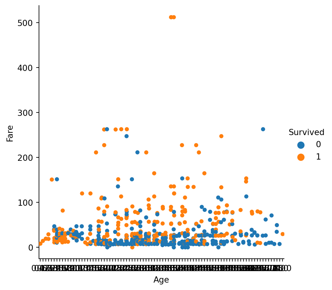
Seems like the older folks were luckier than the younger ones

Code

import matplotlib as mpl
import matplotlib.pyplot as plt
import seaborn as sns

sns.catplot(data = train_eda, x = "Age", y = "Fare", hue = "Survived")
            
plt.show()

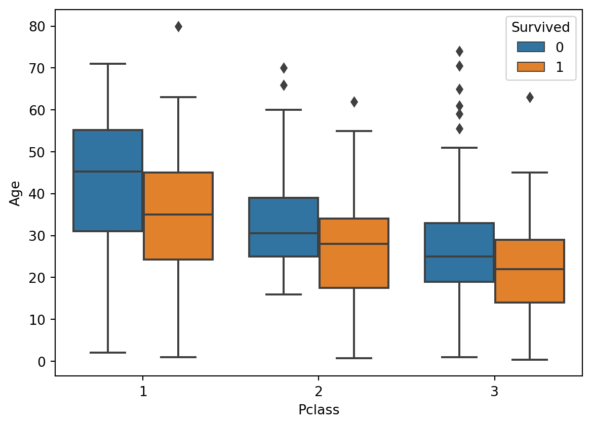
Distinction between Class 1 and Class 3 is clear - poorer folks in Class 3 were younger (mean being just under 30 years) than the richer folks in Class 1

Code

plt.clf()
sns.boxplot(data = train_eda, y = "Age", x = "Pclass", hue = "Survived")
plt.show()

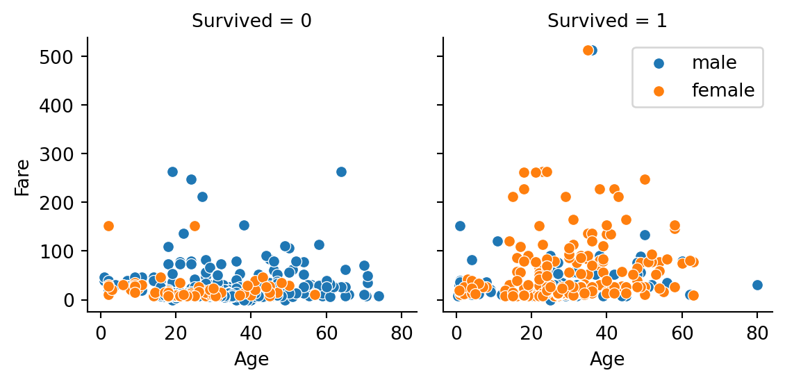
Below graph shows us that among the survivors, there were a lot more women than men survived the disaster.

Code

plt.clf()
plot = sns.FacetGrid(data = train_eda, col = "Survived", hue = "Sex", col_wrap = 2)
plot.map(sns.scatterplot, "Age", "Fare")
plot.axes[-1].legend()
plt.show()

<Figure size 672x480 with 0 Axes>

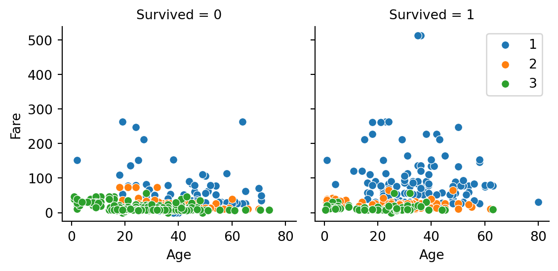
We continue to notice the clearer skew towards Class 1 (richer) compared to Class 3 (poorer)

Code

plt.clf()
plot = sns.FacetGrid(data = train_eda, col = "Survived", hue = "Pclass", col_wrap = 2)
plot.map(sns.scatterplot, "Age", "Fare")
plot.axes[-1].legend()
plt.show()

<Figure size 672x480 with 0 Axes>

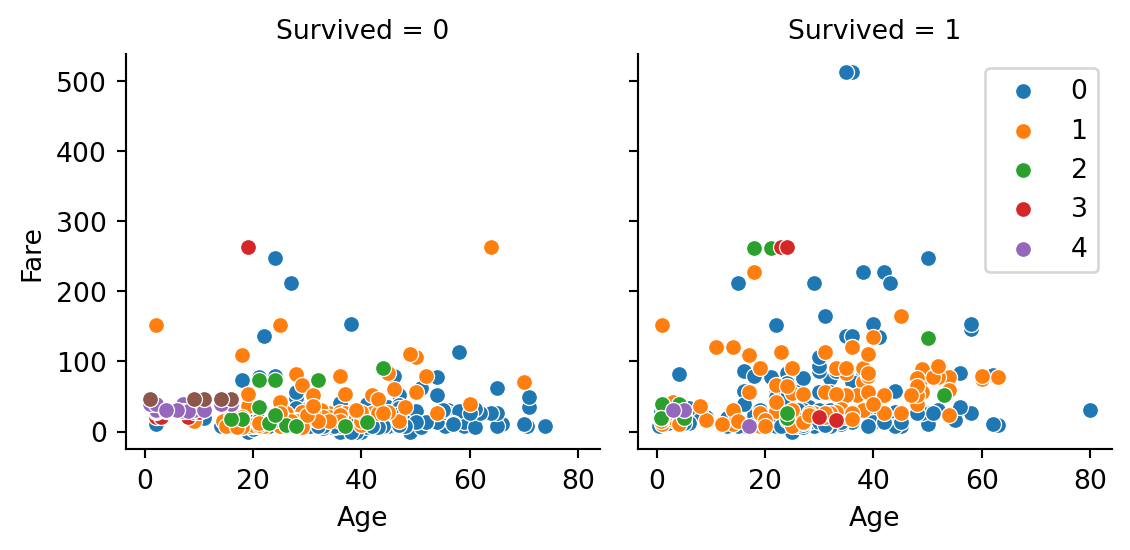
Code

plt.clf()
plot = sns.FacetGrid(data = train_eda, col = "Survived", hue = "SibSp", col_wrap = 2)
plot.map(sns.scatterplot, "Age", "Fare")
plot.axes[-1].legend()
plt.show()

<Figure size 672x480 with 0 Axes>

roughspace

Code

train_df = pd.get_dummies(train_eda, columns = ["Sex", "Embarked"])

train_df.info()

<class 'pandas.core.frame.DataFrame'>
RangeIndex: 891 entries, 0 to 890
Data columns (total 11 columns):
 #   Column      Non-Null Count  Dtype  
---  ------      --------------  -----  
 0   Survived    891 non-null    int64  
 1   Pclass      891 non-null    int64  
 2   Age         714 non-null    float64
 3   SibSp       891 non-null    int64  
 4   Parch       891 non-null    int64  
 5   Fare        891 non-null    float64
 6   Sex_female  891 non-null    uint8  
 7   Sex_male    891 non-null    uint8  
 8   Embarked_C  891 non-null    uint8  
 9   Embarked_Q  891 non-null    uint8  
 10  Embarked_S  891 non-null    uint8  
dtypes: float64(2), int64(4), uint8(5)
memory usage: 46.2 KB

And day 2 comes to an end🤷‍♂️

Day 4: The Titanic Dataset

Importing libraries and reading the data

Rearranging train dataset

EDA

roughspace

Rearranging `train` dataset