TidyTuesday NYT Bestsellers list

tidytuesday
R
Author

Me

Published

June 1, 2022

Tidy Tuesday, Week 19 (2022)

“Learn by practice!” is a maxim that every coder/analyst agrees upon. One of the admirable initiatives by the R/ RStudio community is Tidy Tuesday - every week a new dataset is released for enthusiasts to dig into. A few days back, an interesting dataset caught my eye - NYT’s Bestsellers List from 1930 to 2021. This one was particularly unique as it mirrored a lot of projects that I’ve been doing on the OTT side as well. So I cracked my knuckles and jumped right in!

Objective

  1. Understanding longevity & seasonality of how books track on the NYT bestseller’s list
  2. Deeper understanding of using customizing themes and fonts on the ggplot package

Loading the data

Starting off by loading the data and the libraries

Code
knitr::opts_chunk$set(warning = FALSE, message = FALSE) 
suppressMessages({
  library(tidyverse)
  library(scales)
  library(knitr)
  library(tidytuesdayR)
  library(forcats)
  library(lubridate)
  library(RColorBrewer)
})

tt_raw <- tt_load("2022-05-10")
--- Compiling #TidyTuesday Information for 2022-05-10 ----
--- There are 2 files available ---
--- Starting Download ---

    Downloading file 1 of 2: `nyt_titles.tsv`
    Downloading file 2 of 2: `nyt_full.tsv`
--- Download complete ---
Code
data <- tt_raw$nyt_titles

What’s in the Tidy Tuesday dataset?

Code
glimpse(data)
Rows: 7,431
Columns: 8
$ id          <dbl> 0, 1, 10, 100, 1000, 1001, 1002, 1003, 1004, 1005, 1006, 1…
$ title       <chr> "\"H\" IS FOR HOMICIDE", "\"I\" IS FOR INNOCENT", "''G'' I…
$ author      <chr> "Sue Grafton", "Sue Grafton", "Sue Grafton", "W. Bruce Cam…
$ year        <dbl> 1991, 1992, 1990, 2012, 2006, 2016, 1985, 1994, 2002, 1999…
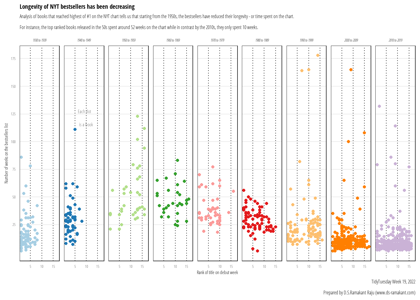
$ total_weeks <dbl> 15, 11, 6, 1, 1, 3, 16, 5, 4, 1, 3, 2, 11, 6, 9, 8, 1, 1, …
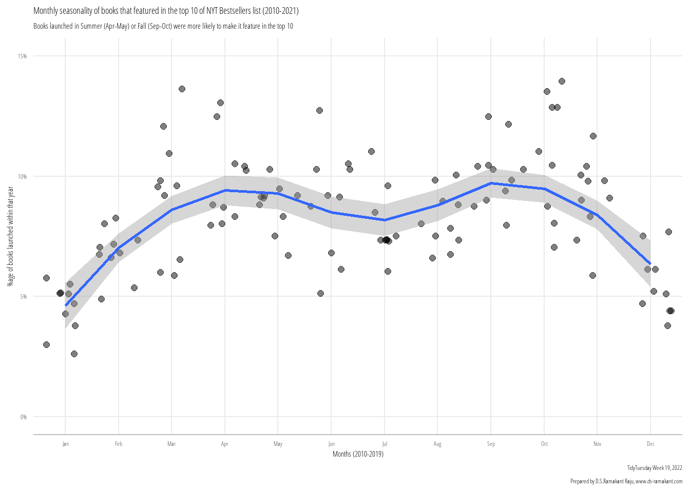
$ first_week  <date> 1991-05-05, 1992-04-26, 1990-05-06, 2012-05-27, 2006-02-1…
$ debut_rank  <dbl> 1, 14, 4, 3, 11, 1, 9, 7, 7, 12, 13, 5, 12, 2, 11, 13, 2, …
$ best_rank   <dbl> 2, 2, 8, 14, 14, 7, 2, 10, 12, 17, 13, 13, 8, 5, 5, 11, 4,…

Exploratory Data Analysis (sort of)

Quick EDA tells us that there the number of books in the #1 spot each year during the 50s have been increasing while the number of weeks they’ve spent on the NYT list has been decreasing. 2020-21 is excluded as I’m breaking up the period into decades for easy analysis

Code
data %>% 
  mutate(decade = factor(10*year %/% 10)) %>% 
  filter(best_rank==1, year<2020) %>% 
  group_by(decade) %>% 
  summarise(avg_weeks = mean(total_weeks),
            no_of_rank1 = n_distinct(title))
# A tibble: 9 × 3
  decade avg_weeks no_of_rank1
  <fct>      <dbl>       <int>
1 1930        17.1          74
2 1940        30.1          59
3 1950        52.4          35
4 1960        45.7          31
5 1970        38.6          46
6 1980        29.5          78
7 1990        25.7          99
8 2000        12.5         220
9 2010        10.3         306

This is a fantastic starting point. Intuitively, this makes a lot of sense. There’s far more competition for the #1 spot in the last 20 years which is driving down the longevity. Compare the 50’s to the 2010’s and the trend is hard to miss. This table is only for the books that made it to the #1 position. But how about the rest of the other books? A visual representation draws the same conclusion more elegantly.

Visualising Longevity

Hat-tip to a few outstanding viz I came across while researching the NYT theme. Bob Rudis’ Supreme Annotations and Rahul Sangole’s Visualizing Correlations

Code
#loading fonts that resemble the NYT viz
#inspired by https://rud.is/b/2016/03/16/supreme-annotations/

library(showtext)
showtext_auto()
font_add(family = "Open Sans", 
         regular = "OpenSans-CondLight.ttf", 
         italic = "OpenSans-CondLightItalic.ttf", 
         bold = "OpenSans-CondBold.ttf")

#changing facet labels as shown here 
#https://ggplot2.tidyverse.org/reference/as_labeller.html
facet_labels <- as_labeller(c(`1930`= "1930 to 1939",
                              `1940`= "1940 to 1949",
                              `1950`= "1950 to 1959",
                              `1960`= "1960 to 1969",
                              `1970`= "1970 to 1979",
                              `1980`= "1980 to 1989",
                              `1990`= "1990 to 1999",
                              `2000`= "2000 to 2009",
                              `2010`= "2010 to 2019"))


#annotations for individual facet as discussed here https://stackoverflow.com/a/11889798/7938068
annot_x <- data.frame(debut_rank = 5, 
                      total_weeks = 111,
                      lab = "Each dot\n is a book",
                      decade = 1940)

graph1 <- data %>% 
  filter(best_rank==1,year<2020) %>% 
  mutate(decade = factor(10*year %/% 10)) %>% 
  ggplot(aes(x = debut_rank, y  = total_weeks))+
  geom_point(aes(color = decade, group = debut_rank))+
  facet_grid(~decade ,labeller = facet_labels)

graph1 <- graph1+
  theme_minimal(base_family = "Open Sans")+
  scale_color_brewer(palette = "Paired")+
  labs(title = "Longevity of NYT bestsellers has been decreasing", 
       subtitle = "Analysis of books that reached highest of #1 on the NYT chart tells us that starting from the 1950s, the bestsellers have reduced their longevity - or time spent on the chart.\nFor instance, the top ranked books released in the 50s spent around 52 weeks on the chart while in contrast by the 2010s, they only spent 10 weeks.",
       caption = "TidyTuesday Week 19, 2022\n Prepared by D.S.Ramakant Raju (www.ds-ramakant.com)",
       x = "Rank of title on debut week",
       y = "Number of weeks on the bestsellers list")+
  theme(panel.border = element_rect(color = "#2b2b2b", 
                                    fill = NA), #borders for each facet panel
        legend.position = "none", #removing legend
        strip.text = element_text(face = "italic"),
        plot.title = element_text(size = 14, face = "bold"),
        panel.grid.major.x = element_line(linetype = "dotted", 
                                          color = "black"),
        panel.grid.minor.x = element_blank(),
        panel.grid.minor.y = element_blank(),
        plot.caption = element_text(size = 12),
        plot.subtitle = element_text(size = 12)) +
  scale_y_continuous(breaks = seq(from = 25, to = 175, by = 25))+
  #annotations by default is applied to all facets
  #for individual facet annotations, check https://stackoverflow.com/a/11889798/7938068
  geom_text(data = annot_x, 
            aes(x = debut_rank, y = total_weeks, 
                family = "Open Sans", alpha = 0.8,
                hjust = -0.2, vjust = -0.2),
            label = annot_x$lab
            )


print(graph1)

Visualising Seasonality

Now lets look at seasonality - is there any trend as far as the launch month is concerned? For the sake of analysis, I’ve truncated the analysis period to 2010 onwards to keep it more relevant and exlcude irrelvant historical data.

Code
graph2 <- data %>% 
  filter(best_rank<11, year> 2010) %>% 
  mutate(month = month(first_week, label = T),
         stage = case_when(year<=2015 ~ "2011-2015",
                           year> 2015 ~ "2016-2020",
                           T ~ "x")) %>% 
  group_by(stage,year,month) %>% 
  summarise(n = n_distinct(title)) %>% 
  mutate(all_titles = ave(n, year, FUN = sum),
         pct = n/all_titles) %>%  
  ggplot(aes(x = month, y = pct, group = 1))+
  geom_point(size = 2, 
             alpha = 0.5, position = "jitter")+
  geom_smooth(se = T) 


graph2 <- graph2+
  theme_minimal(base_family = "Open Sans")+
  scale_color_brewer(palette = "Paired")+
  labs(title = "Monthly seasonality of books that featured in the top 10 of NYT Bestsellers list (2010-2021)", 
       subtitle = "Books launched in Summer (Apr-May) or Fall (Sep-Oct) were more likely to make it feature in the top 10",
       caption = "TidyTuesday Week 19, 2022\n Prepared by D.S.Ramakant Raju, www.ds-ramakant.com",
       x = "Months (2010-2019)",
       y = "%age of books launched within that year")+
  scale_y_continuous(labels = label_percent(accuracy = 1),
                     breaks = seq(from = 0, to = 0.2, by= 0.05), 
                     limits = c(0,0.15))+
  theme(axis.line.x = element_line(color = "grey"),
        panel.grid.minor.y = element_blank())

graph2

This is a fairly straightforward and replicable analysis. If you’re a #TidyTuesday fan please feel free to share your work in the comments below